
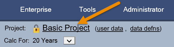
Enersight has a number of options that can be used to optimally solve the production network. These options affect calculation scope and performance. The solver type can be selected under the Project Settings which can be accessed most easily by clicking on the project name:
But also under the Data menu:
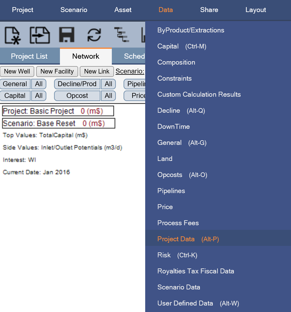
Click image to expand or minimize.
Or using the default shortcut: Alt-P.
In Enersight 2.16, Network Solver selection can be found in the Network Solver Settings section of Project Options.
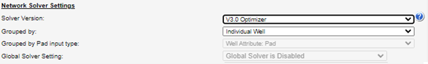
Solver selection has been broken down into the Solver Version, and the Grouped by option, which is how assets are grouped when considered by the solver.
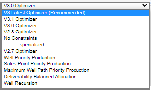
Solver Version
There are currently 10 Solver Versions available, with 6 of these being specialized solvers for unique use cases. There is a new option, V3.Latest Optimizer (Recommended) which will ensure that your project is always using the latest solver when a new version is released (in the future the new solver V3.2 Optimizer for example, will be adopted by the project when it is opened in the new version of Enersight). Of course, if a new solver doesn’t meet your needs, you can always revert to a prior version.
Grouped By and Grouped By Pad Input Type
Assets can be grouped by Individual Well (effectively no grouping), Flows To (grouped by the node assets flow to in the Network), or Pad in the new V3.1 Optimizer. The V2.7 Optimizer has the additional option of Equal Well Constraints.
When grouped by Pad, you can choose how an asset’s Pad is defined using the Grouped by Pad input type’ dropdown. You can either use the Pad Property (found in an asset’s General input modal) or a User Data Field.
Note that in previous versions, the Equal Well Const by Pad solver option was effectively a Group by Flows To option. The V3.1 Optimizer offers more flexibility in how assets can be grouped.
The Global Solver Setting is described below in the 2.8 Optimizer section.
V3.1 Optimizer
The V3.1 Optimizer is not a revolution, it builds on the concepts introduced in the V3.0 Solver, improves upon some of them, and adds some additional capabilities.
Highlights include a true Group by Pad option, support for negative production, and improved pipeline split logic. Note that if your project is currently using the V3.0 solver, it will automatically be updated to use the V3.Latest solver.
- Group by Pad: in previous versions, the ‘equal well const by Pad’ solver types behaved more like a ‘Flows to’ optimization. In the V3.1 Optimizer, the solver groups assets for the network optimization using either the Pad metadata on an asset or by a user-selected User Data field. Assets with blank values will be treated as individual wells.
- Negative production support: production values can now be entered as negative values and will be incorporated into the network optimization problem. Note that constraints with negative values are not supported and that unintended behaviors may be seen when negative flows are combined with pipeline priorities and splits as well as if net negative flows are seen at aggregation points (e.g., facilities).
- Solver selection improvements in Project Settings: solver selection has been split into the version and grouping type (individual asset, Pad, Flows To), and the type of Pad grouping (when applicable) to simplify the options. Additional options such as using the Lindo or Global solver are available only when appropriate.
- Pipeline split precedence: in the V3.1 Optimizer, when a product specific pipeline exists, this will take precedence over any other pipeline type. Previously when a constraint was hit, remaining product could flow down a more generic pipe, but that is no longer the case, which is similar to the previous Remain pipeline behavior.
- A calculation warning will now be raised if we detect a pipeline split that includes product-specific and generic pipelines (e.g. an Oil and an All pipeline). We recommend that you change any All pipelines in this situation to a Remain pipeline.
V3 Optimizer
From Version 2.14 onwards, our new V3 Optimizer is the default option assigned to newly created projects. This solver is in general substantially faster and more transparent than the previously available Full Optimization methods. Pre-existing projects may also have this solver assigned to it (or its Equal Well Const By Pad twin), whereby pending the particular pipeline configuration, some adjustments may be required in order to facilitate getting the same answer. A testing and review process is recommended when converting so as to best identify where changes may be required or determinism introduced causing the more robust selection of candidates. Refer to How to Swap Solver Types for a recommended procedure on converting between options.
This solver builds upon the previously available Full Optimization methods with a re-formulated conceptualization of the network that retains the existing goal of optimizing the total hydrocarbon production. Acting similarly to previously available solvers, the method accounts for all the constraints, extractions, yields, shrinkages in the network across the possible paths that the production may flow through to find the best solution given the rules.
The reformulation of the problem negates the need for a global solver whilst still enabling the TRUE optimum solution to be presented for any number of the available 18 products, paths, constraints and transformations. Each time step is solved in sequence with its own conditions / topology allowing for correct cumulative deferment effects on the wells.
The default optimization weightings from the previous solver have been retained, including a slight bias against non-hydrocarbon products. Please contact Quorum if you wish to discuss changing these weightings for your project.
A series of deterministic rules have been introduced within the V3 Solver method to better address the challenge of problem spaces not being fully defined, resulting in an infinite number of possible solutions. These rules remove some of the apparent randomness in individual well performance seen in previous solvers and are specifically associated with Pipeline Priorities and Well Selection for shut-in when constrained:
Pipeline Priorities previously influenced the objective value being maximized based upon their delta from 10 and hydrocarbon throughput. This enabled behaviour such as adjusting the priority to nudge the solution in the desired direction. Within the V3 solver, the split flows are evaluated at each level and will fill the ‘best’ priority options in first regardless of absolute priority value e.g. it doesn’t matter if it is 1, 7 and 9 or 8, 9 and 10. Only if something downstream is identified as blocking the flow will the better priority options not be filled first so as to achieve its goal of greater overall hydrocarbon flow. In cases where the priority of two (or more) pipelines from the same facility are equal, the solver will endeavour to fill equally, again pending downstream limitations.
The effect of network constraints on individual wells has also been revised with an adjusted selection of which wells will be shut in when encountering this element. The revised ranking order for which wells will be shut-in for a given sub-section of a network where a constraint is operating is below:
- Oldest Asset Start Date. This metric has been selected as a good proxy for your best NPV producing wells as you probably don’t want to shut-in your newest and most likely, highest, producers. This also this helps ensure that if a well has a limited time royalty holiday, that well is prioritized above others
- Previous Rate of Take: Whereby a penalty function is assigned against a well that was fully shut in within the previous timestep to avoid noisy swapping between roughly equivalent wells between each timestep
- Potential Production whereby the lowest potential wells are shut in first
- Name on an alphabetical basis
If you wish to use the V3 Optimizer, but don’t want to use the default shut-in ranking methodology, please contactQuorum to discuss customizations possible.
Additional to the deterministic rules, within the new V3 solver there were a few limitations introduced relative to the previous solvers:
- Extraction values above 100% will result in an infeasible outcome and no solution. An error is written to the calculation log advising of this, the offending asset(s) and that if such functionality is required that swapping over to a 2.8 Solver is recommended.
- Negative production is not supported by the V3 Solver. A warning has been added in calc log per timestep where negatives occur. Actual behaviour below:
- Negative Production Potential is treated as 0 within the solver and thus presumed to occur at a 100% ROT (or as determined by other products constrained on the same well)
- Subsequently to the ‘optimized’ results being passed back, the negatives are rolled through the network presuming that 100% ROT along with the solved ROT for other products.
- Negatives will flow through the network based upon proportional flow e.g. If 25% of the positive production goes here based upon the optimizer, then 25% of the negative will also flow there
- Constraints are thus not filled in any path where negatives may occur, even if options exist within the model to fill it (i.e. extracting additional un-used potential from shut-in wells or from shifting production flows away from lower priority pipes)
- Where used within a model which simply aggregates or where no constraints are present, it is likely that the negatives will cause behaviour as expected.
Within a V3 Solver model, the resolved production at Facility X would be 60 bbl/d as Well B is not considered during the solve and thus Well A only sends 80% of its available potential to meet the intended capacity of 80 bbl/d. This amount however is then decremented by the negative rates of Well B towards this lower total.
In a 2.8 Solver model, the resolved production at Facility X would be 80 bbl/d as the solver considers the negative potential as it evaluates against the constraints.
- Energy Constraints with WI Flow only pipelines and gas compositions with Heating Value Overrides are not supported by the V3 Solver. An error is written to the calculation log advising of this and that if such functionality is required that swapping over to a 2.8 Solver is recommended.
Finally, the V3 solver also resolves a couple of bugs identified within previous solvers whereby:
- Incorrectly defined split flow percentages at facilities will no longer cause local losses or gains on subsequent nodes (correct at the scenario level), the new behaviour rather is that appropriate errors are reported for infeasibility whilst providing the following outcomes:
- Where less that 100% availability is collectively defined, the solution is infeasible and will return 0 with errors
- Where there is greater than 100% absolute deliverability collectively defined, then the solution is infeasible and will return 0 with errors
- Where there is greater than 100% maximum availability collectively defined, then the highest priority flows will be filled as per normal optimizer solutions up to the maximum percentage for that path, with adjustments only made where downstream limitations become prohibitive
- Products which have been removed from the flow path may still be constrained if they re-appear through a product transformation e.g. both injected water and normal water are associated with a well. Within the network, the injected water may be flown in an alternative direction to the normal water. If that normal water product is transformed into injected water via an Extraction input at a facility subsequently to that split, then it now will respond to constraints as would be expected in the normal case
No Constraints
This option turns the solver off and ignores any system constraints. Wells can produce to their full capacity throughout the network.
Full Optimization (2.8)
The full optimization (2.8) was the main solver prior to Version 2.14.
This solver builds a large slightly Non-Linear Programming model of the network and then proceeds to optimize the total hydrocarbon production. The model that is built takes into account all of the constraints in the network and the points in the network where production can flow in multiple paths and finds the overall best solution given the constraints.
This solver will find the TRUE optimum solution to the network in the face of any topography, any number of products, and any number of constraints.
All 18 products are modeled at the same time, taking into account the constraints entered at facilities and pipelines, the topography of the network is allowed to change at each time step, and the compositional flow of each well can be unique.
In a constrained network with an infinite number of possible solutions to meet the constraints entered, the selected solution can appear rather random at the individual well level. Wells that are on production one month are given a slight edge in the model to continue production.
This model also has a slight bias against non-hydrocarbon production (such as water), so that in a case where two wells can produce to a gas constrained facility, it will select the low water cut well first, for instance.
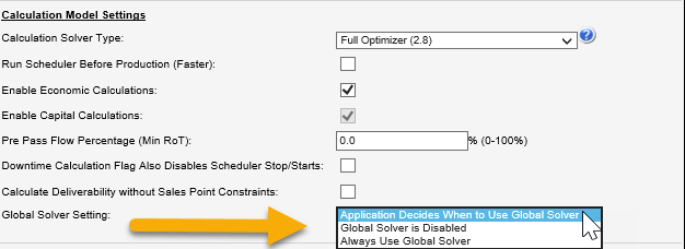
Global Solver in Full Optimization
By default, the Full Optimization (2.8) uses the "Global Solver" on an evaluated basis. This solver is a robust solver that improves the solution for complex (split flow) networks. As a more robust solver, it also increases the calculation time. If you are looking to improve the calculation time, you can test your project with the Global Solver turned off. The solution should still be reasonable, and the calculation time much quicker. Global Solver Settings can be adjusted using the drop down box under the Calculation Model Settings:
Click image to expand or minimize.
Equal Constraint by Pad
This solver variant is based on the above Optimization Solver methods, but all constrained wells that flow to the same target facility will be cut back equally. This produces a non-optimal solution but can meet certain business constraints. The results from this solver will look more intuitive, and better behaved than the individual well optimization as production is not radically changing month to month.
If wells flow to an individual pads with a few wells each, you may still see rapid production switching by facility.
Well Priority Production
This solver uses a much more basic algorithm to assign the production to the network. To start, all of the possible paths from well to the Scenario are calculated. A well that can pass through two different paths when it encounters a split point generates a path for both directions.
Each well is assigned a priority STARTING AT THE WELL that represents each pipeline between the well and the scenario. Each segment generates a number equal to (10 – Pipeline Priority), so a well that passes through 3 pipelines, all of which are set to priority 10 (the default) will get a priority of 0.0.0.
If the pipeline directly leaving the well was changed to priority 4 then this priority number would become 6.0.0.
Wells with the same priority are ranked in the order that they were created (essentially randomly, although this order is consistent between runs).
All of the paths are then ranked against each other from highest to lowest (6.0.0 goes before 0.0.0).
Well production is then layered into that path for each well, until all of the wells production has been assigned to the network. If there is not room through any of the paths then the well is curtailed to meet the entered Constraints of the network.
This is done for each product in the model. This can mean that although there is room for the gas, the water production may then limit the well further at a later point of the calculation. The algorithm does not then try and re-assign the missing gas production, therefore mathematically sub optimal answers are possible when dealing with multiple product constraints.
Re-convergent split flow (where two paths separate then come back together later in the network), mixed with constraints at those nodes is also a situation that can have sub optimal answers and is not recommended for this solver.
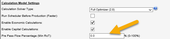
Other Options for the Path Priority Solvers include Pre Pass Flow Percentage (Min RoT): This is a percentage of the production from all wells that is attempted to be flowed through the network as a first pass. Then enables all wells to have a higher chance to flow some portion of their potential before the network is completely full. Setting this to either 0% or 100% would have no effect on the network.
This solver is the same as the Well Priority Solver, except that the priorities are assigned a priority based on the highest priority pipeline at any point between the well and the scenario.
Wells with 3 pipelines with priorities 6,0,0 or 0,6,0 or 0,0,6 all would receive the same priority.
Sales Point Priority Production
This solver is the same as the Well Priority Solver, except that the priorities are assigned from the final nodes of the network upstream towards the well.
This has the impact of defining the priorities more of a pull rather than a push model in the network, letting you choose which of the incoming pipelines to prioritize at a given node.
Deliverability Balanced Allocation
This solver uses an algorithmic solution to allocate production based on prioritization of pipeline connections. This solution works great where you have an idea of the individual well/pipeline priorities in your network.
At each point in the network, the available constrained production room is allocated based on a simple weighting formula. The weighting factors are a function of the inflowing pipeline priorities. The weighting factor is equal to 10 minus the pipeline priority. A priority 2 pipeline has a weighting of 8, while a priority 10 has a weighting of zero. The allocation for each pipeline is equal to the weighting factor for that pipeline divided by the sum of all the weighting factors.
After each inflowing node has had its weighted chance to provide production, any unused allocation is repeatedly offered to any remaining inflows that have unused deliverability. This weighting is done at each individual node throughout the network starting with the most downstream nodes.
For example, if a priority 1 pipeline flowing into a facility with a priority 2 pipeline, then they will get allocated 53%: (10-1) / ((10-1) + (10-2)) and 47%: (10-2) / ((10-1) + (10-2)) respectively.
For three pipelines, with priorities of 2, 6, and 8, their allocation will be 57%, 29% and 14% respectively.